User Manual
Load LOG file
A Safecast layer (a LOG file) can be loaded from the main toolbar by
 Import Log file as new layer. An input file is loaded
into QGIS as a new vector point layer. The name of new layer
corresponds with the input file (without LOG extension). Measured
points are categorized based on the dose rate (ADER)
value (see Introduction). ADER is calculated from CPM (from the 5 second pulse count data by default) using the conversion factor (1/334) provided by Safecast.
Import Log file as new layer. An input file is loaded
into QGIS as a new vector point layer. The name of new layer
corresponds with the input file (without LOG extension). Measured
points are categorized based on the dose rate (ADER)
value (see Introduction). ADER is calculated from CPM (from the 5 second pulse count data by default) using the conversion factor (1/334) provided by Safecast.
During import, the plugin also checks the data and drops points with following values:
- HDOP=9999 or SAT<3 as these points have completely wrong position
- latitude and longitude are both zero value (see Null Island for more details)
The plugin also checks and fixes date - as sometimes (maybe because of bad GPS signal or some other errors) the data contain meaningless date values The year value cannot be less than 2011 and more than current date. The Fukushima Daiichi nuclear disaster happened 11 March 2011 and Safecast was established after the accident so there cannot be Safecast data before 2011. The plugin uses correct date values (the time is in most cases correct) from the rest of the file and fixes the incorrect ones (no problem with measuring over midnight).
By default, the points are categorized in a range from 0.08 to 5.00 microSv/h. See the figure below.
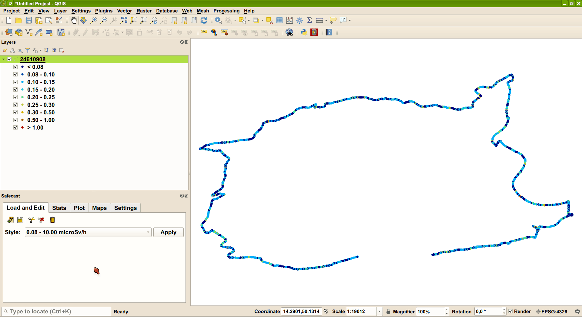
Figure 1: Loaded Safecast layer with the default style applied.
The alternative style (0.05 - 200.00 microSv/h) can be chosen from the style selector and activated for a selected layer by Apply button.
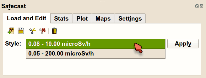
Figure 2: Style selector to apply predefined point styles.
The default style (0.08 to 5.00 microSv/h) was designed for measurements at low dose rate levels (natural background) with more categories for lower values to distinguish natural background variations.
Note
The color ramp is derived from the default SAGA GIS color style which has proved to be optimal for most of our tasks.
The second available style (0.05 - 200.00 microSv/h) was designed to mimic the Safecast Tile Map default style. This is useful for areas with higher dose rate levels like Fukushima or Chernobyl.
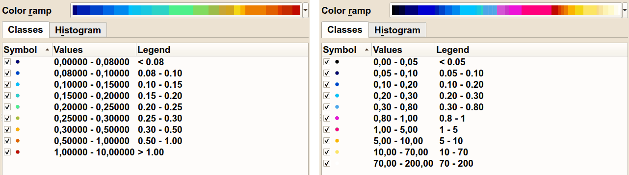
Figure 3: Predefined point styles - 0.08 to 5.00 microSv/h on the left and 0.05 - 200.00 microSv/h on the right.
Tip
If none of above mentioned styles fits your needs and you want to
create your own style, then use native QGIS styling capabilities to be
available in the programme (right click on layer name, choose
Properties from the context menu, then go to Style tab).
Layer statistics
“Stats” tab provides basic statistics of selected Safecast layer:
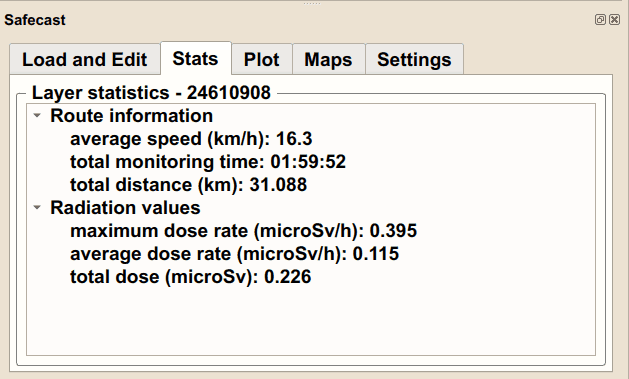
Figure 4: Layer statistics tab.
Layer statistics Route information
- average speed (km/h)
- total monitoring time
- total distance (km
Radiation values
- maximum dose rate (microSv/h)
- average dose rate (microSv/h)
- total dose (microSv)
Layer graph
“Graph” tab shows you a simple dose rate graph which can be useful for quick checks and easy identification of hotspots.
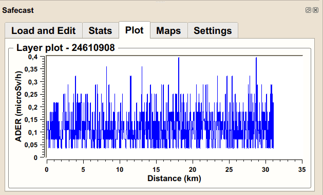
Figure 5: Layer graph tab.
Add background map (Google, Bing, OpenStreetMap or offline)
By default, there is no background map - you need to add it from offline data (vector or raster files) or to add a layer from online map service like Google or OpenStreetMap, using OpenLayers plugin.
Go to :
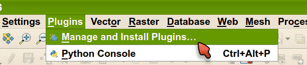
Figure 6: Plugins menu.
Write openlayers in Search field, select OpenLayers Plugin and
start installation, using Install Plugin button.
Note: currently, OpenLayers Plugin for QGIS3 is still marked as “experimental” so you have to tick the checkbox “Show also experimental plugins” in plugin manager settings in order to be able to see and install OpenLayers plugin.
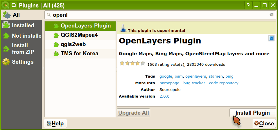
Figure 7: OpenLayers Plugin installation.
Go to the menu and choose
the map layer you want to add - in this case it is Google Hybrid:
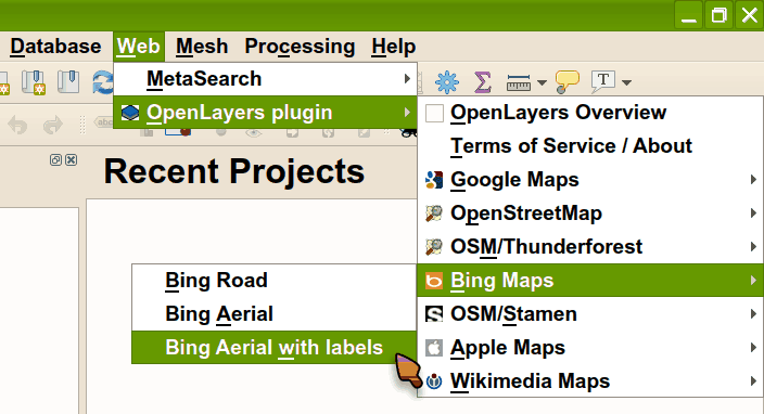
Figure 8: OpenLayers Plugin - add layer to map.
The map layer loads on the top, so it covers your data:
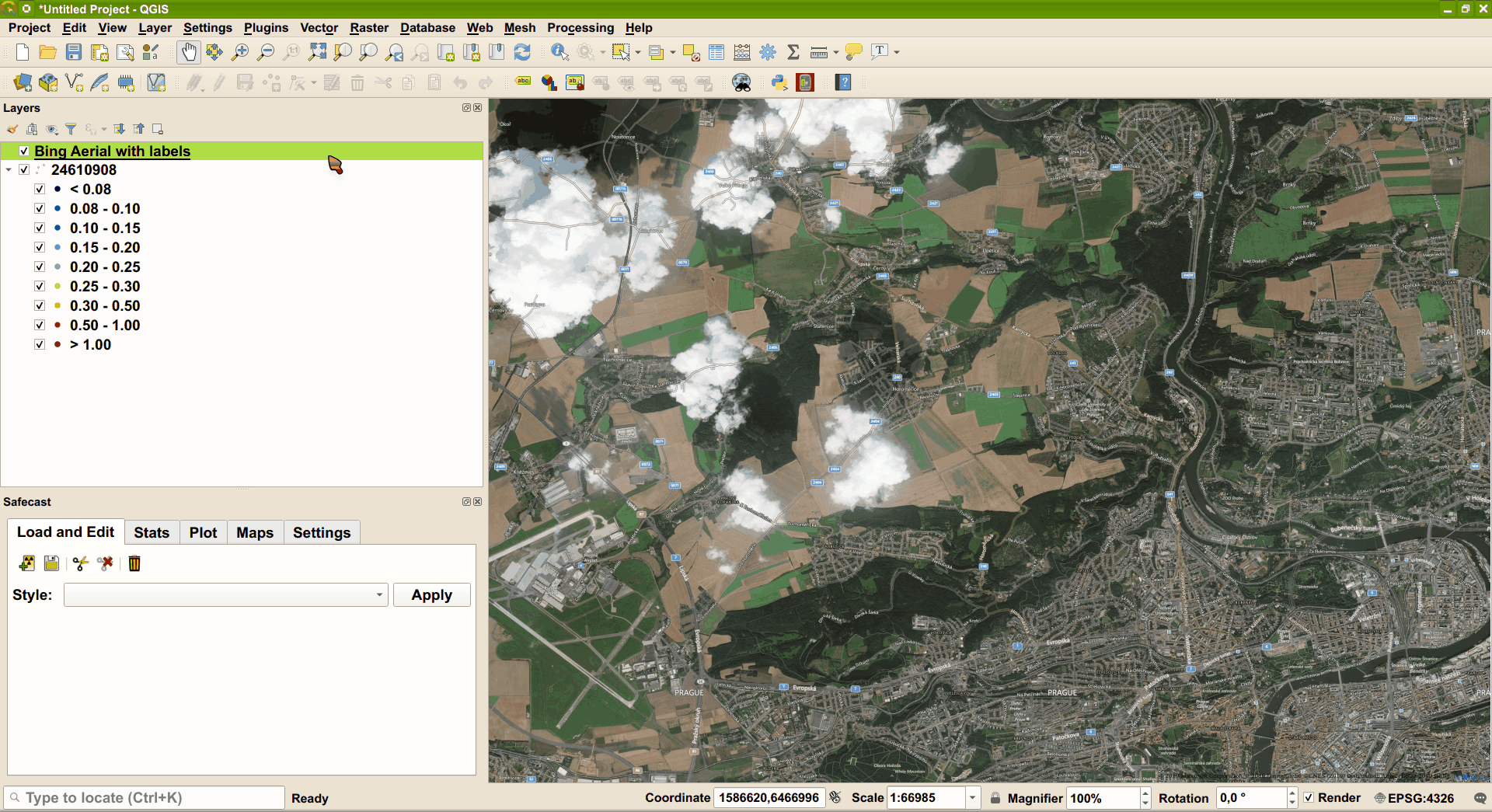
Figure 9: Newly added layer covers your data.
To fix this, you just need to drag the background map layer to the bottom with the mouse.
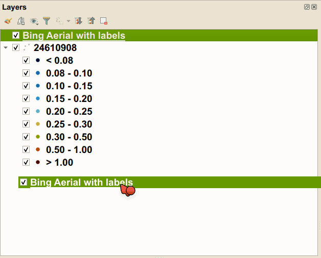
Figure 10: Drag the background layer to the bottom.
Finally you get your measurements to be displayed on the Google map layer.
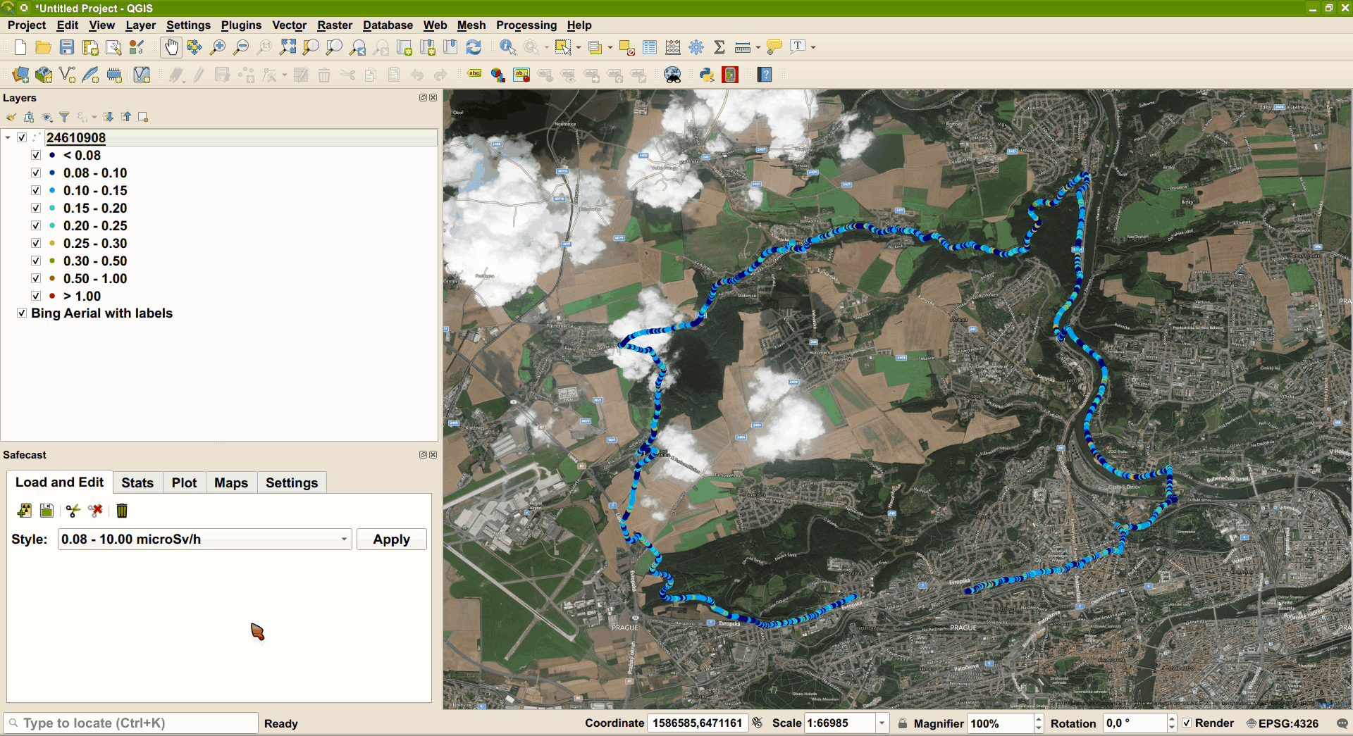
Figure 11: Loaded Safecast layer with the default style applied.
Offline maps
QGIS can use various offline data sources. Depending on type of your data (raster / vector), level of details and spatial extent, the time needed to refresh the map window after panning or zooming can increase significantly.
Browse attribute data
You can display all loaded data from the LOG file in a table form - in GIS programs; it is called Attribute table.
Note
This is not a feature of Safecast plugin - it is a standard, built-in QGIS feature.
In Layers Panel select particular layer, using a mouse. Then click a
right mouse button to show the context menu and select Open
Attribute Table.
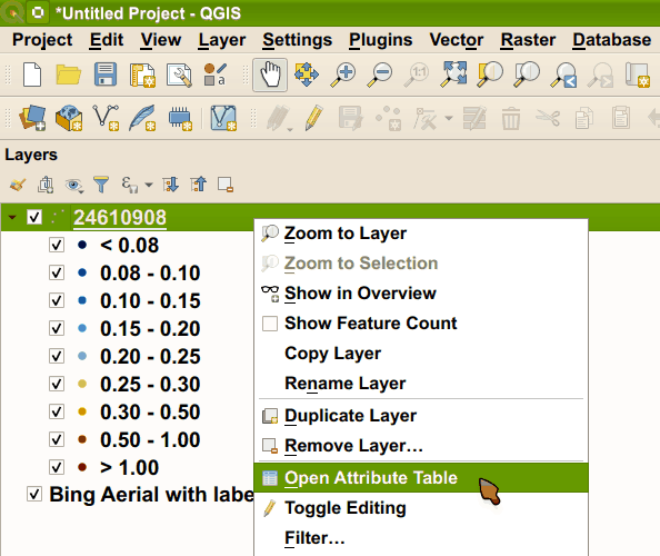
Figure 12: Opening the attribute table.
Then the attribute table appears:
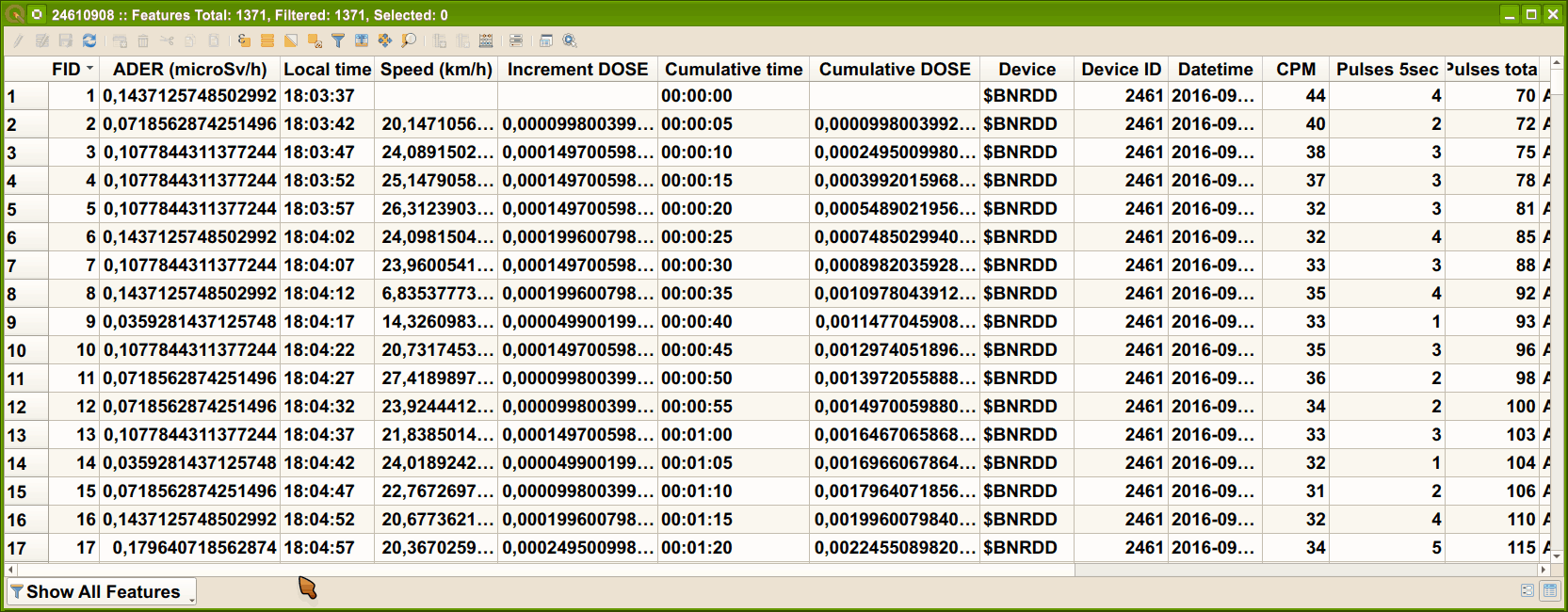
Figure 13: Attribute table data.
The table contains both all data imported from the bGeigie LOG file and several additional ones calculated by the plugin - dose rate, local time etc.
Delete measured points
The plugin allows a user to select and remove particular measured points and then to save the corrected set as a new LOG file for uploading to Safecast web map. No modification of the data values is possible.
There are various reasons for using this feature:
- After returning home, you forgot to switch off your bGeigie. More than half of the data uploaded to Safecast map to be unnecessary.
- It is comfortable to switch on bGeigie at home, but you do not want to let all people know the exact location of your home. You need to begin either data measurement later, or to end it earlier.
- Some points have missing or incorrect coordinates; you want to drop them from the dataset.
- You have one LOG file containing several trips measured under different conditions. You need to split them into separate files for an upload to Safecast API and to provide a different description (height, facing etc.) for each one.
First select the layer with loaded LOG data you want to trim:
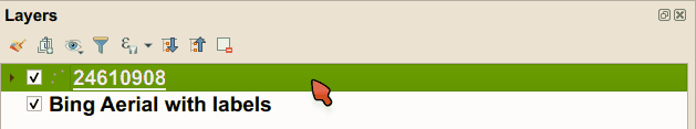
Figure 14: Select the layer to be trimmed.
Then use the  Select features to cut button to select
the points, you want to remove by simply drawing a rectangle over
them:
Select features to cut button to select
the points, you want to remove by simply drawing a rectangle over
them:
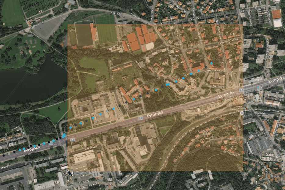
Figure 15: Select features to cut.
Tip
Use the panning and zooming tools to zoom or move the map to a desired area and scale. Only while activating panning tool, you can also use a mouse wheel to zoom in or out and arrow keys to move.
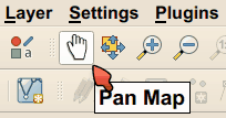
Figure 16: QGIS panning and zooming tools.
All selected points will turn yellow:
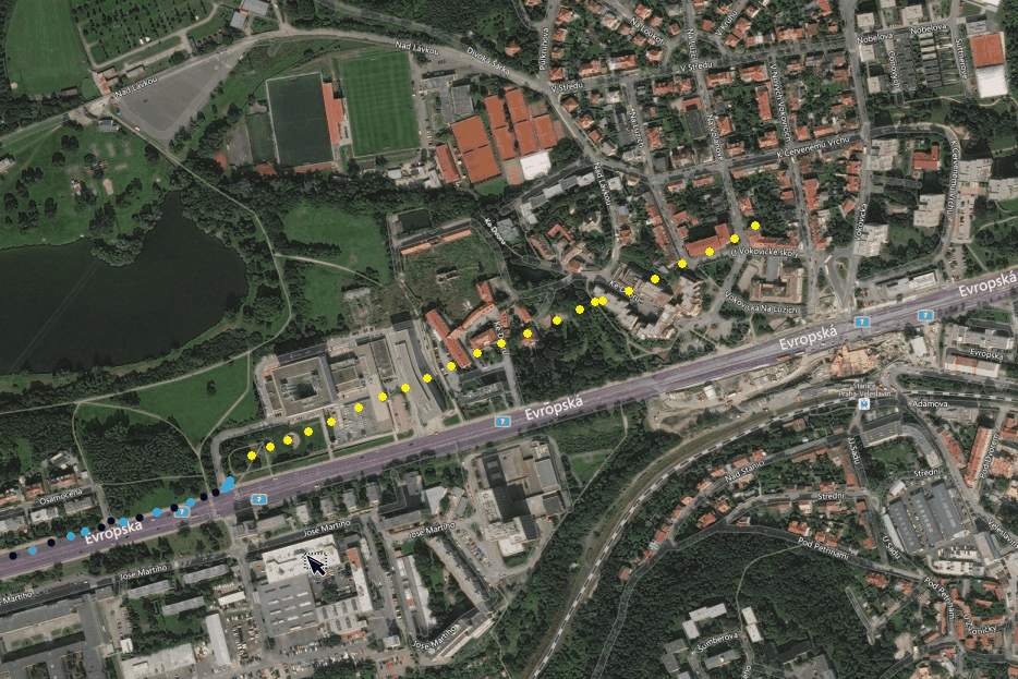
Figure 17: Selected points are highlighted with yellow color.
Click the  Delete selected features button to delete
selected points and confirm the deletion:
Delete selected features button to delete
selected points and confirm the deletion:
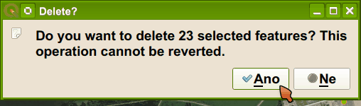
Figure 18: Deleting points.
Then the selected points are deleted.
Important
Since the plugin loads the data in the memory (a separate working file is planned for future versions) any changes does not affect the source LOG file. When a user wants to keep changes in the LOG file, it is necessary to save them into a new LOG file.
Save changes into new LOG file
Click the  Save layer as new LOG file button to save the
data as a new LOG file. We recommend to use a different file name. For
example, the source data file is 24610908.LOG; we save the trimmed
LOG file as 24610908_upload.LOG. By this means it marks that this
file is ready for an upload to Safecast API.
Save layer as new LOG file button to save the
data as a new LOG file. We recommend to use a different file name. For
example, the source data file is 24610908.LOG; we save the trimmed
LOG file as 24610908_upload.LOG. By this means it marks that this
file is ready for an upload to Safecast API.
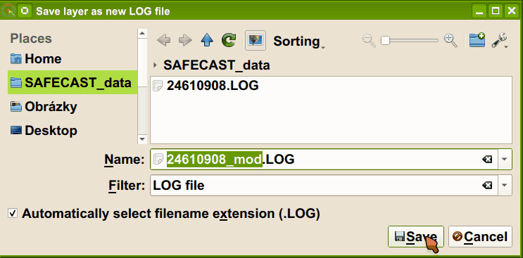
Figure 19: Save layer as LOG file.
Note
While saving into LOG files, additional columns (see [1]) will not be saved. The only way to keep them is to save the layer in other format selected from the context menu in QGIS, because the plugin allows you to save them only as a LOG file.
How to show values of particular point using Identify Features tool
If you want to show an exact value (dose rate, CPM and others) for a
particular measured point, then Identify Features is the right tool for you.
Note
This is not a feature of Safecast plugin - it is a standard, built-in QGIS feature.
First select the layer with the loaded LOG data you want to identify:
Figure 20: Select the layer to identify.
Then activate the Identify Features tool in the main toolbar:
Figure 21: Activate Identify tool.
If you cannot see separate points, then use the panning and zooming
tools mentioned in Delete measured points
section to achieve a needed map scale. Then activate Identify tool
again. Click on the point:
Figure 22: Using Identify tool.
And QGIS will display Identify Results window with all data (attributes) for the selected point.
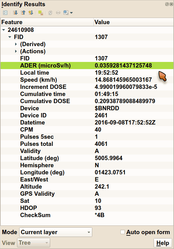
Figure 23: Identify Results window.